TikZ
 とは
とは
 とは、
とは、 文書内で高品質な図を作成するための強力な描画パッケージです。は数学記号の文書を作成する際に広く使用されている電子組版システムで、TikZはその中で図やグラフィックを直接コード化して描画するために使われます。例えば、以下のようなコマンドを使用して簡単な図形を描くことができます。
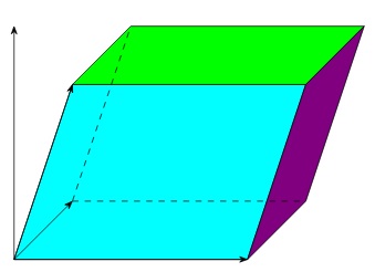
平行六面体
コード
\begin{tikzpicture}
\draw[fill=magenta] (0,0)--(4,0)--(5,3)--(1,3)--(0,0);
\draw[fill=cyan] (5,3)--(1,3)--(2.2,4.2)--(6.2,4.2)--(5,3);
\draw[fill=lime] (4,0)--(5,3)--(6.2,4.2)--(5.2,1.2)--(4,0);
\draw[dashed] (2.2,4.2)--(1.2,1.2);
\draw[dashed] (0,0)--(1.2,1.2);
\draw[dashed] (1.2,1.2)--(5.2,1.2);
\end{tikzpicture}
出力画像

その他
ベクトル座標付き平行六面体
コード
\usetikzlibrary{arrows.meta}
\begin{tikzpicture}
\draw[fill=cyan] (0,0)--(4,0)--(5,3)--(1,3)--(0,0);
\draw[fill=green] (5,3)--(1,3)--(2,4)--(6,4)--(5,3);
\draw[fill=violet] (4,0)--(5,3)--(6,4)--(5,1)--(4,0);
\draw[dashed] (1,1)--(2,4);
\draw [->, >={Stealth[round]}] (0,0)--(1,1);
\draw [->, >={Stealth[round]}] (0,0)--(4,0);
\draw [->, >={Stealth[round]}] (0,0)--(1,3);
\draw [->, >={Stealth[round]}] (0,0)--(0,4);
\draw[dashed] (1,1)--(5,1);
\end{tikzpicture}
出力画像
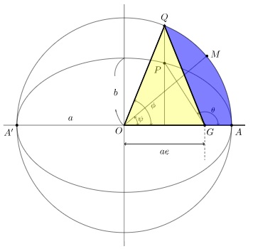
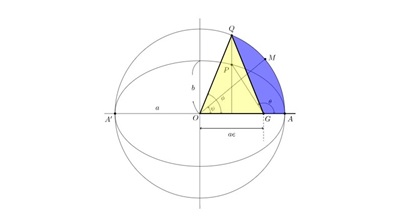
惑星の楕円軌道運動
コード
\usetikzlibrary{angles, quotes}
\begin{tikzpicture}
\draw (0,0) circle[radius=4cm];
\draw (0,0) circle[x radius=4cm, y radius=2.5cm];
\draw (-4.5,0) -- (4.5,0)
\draw (0,-4.5) -- (0,4.5)
\draw (0,0) -- (1.5,3.7)
\draw (1.5,3.7) -- (3.0,0)
\draw (4.5,0) coordinate (A) -- (0,0) coordinate (B) -- (40:4) coordinate (C) ;
\draw pic["$\psi$", draw, <->, font=\footnotesize, angle eccentricity=1.3, angle radius=0.5cm] {angle=A--B--C};%
\draw (4.5,0) coordinate (A) -- (0,0) coordinate (B) -- (68:4) coordinate (C) ;
\draw pic["$\phi$", draw, <->, font=\footnotesize, angle eccentricity=1.3, angle radius=1.0cm] {angle=A--B--C};%
\foreach \P in {(1.5,3.7),(3,0),(3.08,2.58)} \fill \P circle[radius=1.5pt];
\draw (4.5,0) coordinate (A) -- (3,0) coordinate (B) -- (56:2.75) coordinate (C) ;
\draw pic["$\theta$", draw, <->, font=\footnotesize, angle eccentricity=1.3, angle radius=0.5cm] {angle=A--B--C};%
\node (O) at (-0.2,-0.2) {$O$};
\node (O) at (3.2,-0.25) {$G$};
\fill (4,0) circle[radius=1.5pt] node[below right] {$A$};
\fill (-4,0) circle[radius=1.5pt] node[below left] {$A^{\prime}$};
\draw (0,0) to[out=160,in=105] (-0.3,0.5);
\draw (0,2.5) arc[radius=0.7, start angle=120, end angle=185];
\node (O) at (-0.32,1.23) {$b$};
\node (O) at (-2,0.25) {$a$};
\draw (1.5,3.6) -- (1.5,0)
\fill (1.5,2.31) circle[radius=1.5pt] node[below left] {$P$};
\node (O) at (3.4,2.65) {$M$};
\node (O) at (1.5,4.0) {$Q$};
\filldraw [fill=blue, opacity=.5, draw=Indigo] (4,0)  arc (0:68:4) --(3,0)--cycle;
\draw[dash pattern=on 2pt off 2pt on 2pt off 2pt] (3,0) -- (3,-1.3);%ダッシュライン
\draw[<->] (0,-0.7) -- (3,-0.7)%左右矢印範囲指定距離
\node (O) at (1.5,-1.0) {$ae$};
\draw[<->] (0,-0.7) -- (3,-0.7)%離心点距離
\coordinate[label=left:] (A) at (0,0); %点Aの定義
\coordinate[label=right:] (B) at (3,0); %点Bの定義
\coordinate[label=above:] (C) at (1.5,3.7); %点Cの定義
\fill[fill=yellow, opacity=.3] (A)--(B)--(C)--cycle; %三角形OQDをyellow(明るい黄色)に塗る
\draw[very  thick] (A)--(B)--(C)--cycle; %三角形ABC
\end{tikzpicture}
出力画像
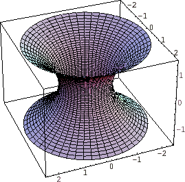
また大変複雑になりますがこれ以外にも次のような興味深い画像の出力も行えます。
Polarizing microscope
コード
\documentclass[11pt]{article}
\usepackage{tikz}
\usetikzlibrary{arrows}
\begin{document}
\begin{tikzpicture}[x={(0.866cm,-0.5cm)}, y={(0.866cm,0.5cm)}, z={(0cm,1cm)}, scale=1.0,
    %Option for nice arrows
    >=stealth, %
    inner sep=0pt, outer sep=2pt,%
    axis/.style={thick,->},
    wave/.style={thick,color=#1,smooth},
    polaroid/.style={fill=black!60!white, opacity=0.3},
    ]
    % Colors
    \colorlet{darkgreen}{green!50!black}
    \colorlet{lightgreen}{green!80!black}
    \colorlet{darkred}{red!50!black}
    \colorlet{lightred}{red!80!black}
    % Frame
    \coordinate (O) at (0, 0, 0);
    \draw[axis] (O) -- +(14, 0,   0) node [right] {x};
    \draw[axis] (O) -- +(0,  2.5, 0) node [right] {y};
    \draw[axis] (O) -- +(0,  0,   2) node [above] {z};
    \draw[thick,dashed] (-2,0,0) -- (O);
    % monochromatic incident light with electric field
    \draw[wave=blue, opacity=0.7, variable=\x, samples at={-2,-1.75,...,0}]
        plot (\x, { cos(1.0*\x r)*sin(2.0*\x r)}, { sin(1.0*\x r)*sin(2.0*\x r)})
        plot (\x, {-cos(1.0*\x r)*sin(2.0*\x r)}, {-sin(1.0*\x r)*sin(2.0*\x r)});
    \foreach \x in{-2,-1.75,...,0}{
        \draw[color=blue, opacity=0.7,->]
            (\x,0,0) -- (\x, { cos(1.0*\x r)*sin(2.0*\x r)}, { sin(1.0*\x r)*sin(2.0*\x r)})
            (\x,0,0) -- (\x, {-cos(1.0*\x r)*sin(2.0*\x r)}, {-sin(1.0*\x r)*sin(2.0*\x r)});
    }
    \filldraw[polaroid] (0,-2,-1.5) -- (0,-2,1.5) -- (0,2,1.5) -- (0,2,-1.5) -- (0,-2,-1.5)
        node[below, sloped, near end]{Polaroid};%
    %Direction of polarization
    \draw[thick,<->] (0,-1.75,-1) -- (0,-0.75,-1);
    % Electric field vectors
    \draw[wave=blue, variable=\x,samples at={0,0.25,...,6}]
        plot (\x,{sin(2*\x r)},0)node[anchor=north]{$\vec{E}$};
    %Polarized light between polaroid and thin section
    \foreach \x in{0, 0.25,...,6}
        \draw[color=blue,->] (\x,0,0) -- (\x,{sin(2*\x r)},0);
    \draw (3,1,1) node {Polarized light};
    %Crystal thin section
    \begin{scope}[thick]
        \draw (6,-2,-1.5) -- (6,-2,1.5) node [above, sloped, midway]{Crystal section}
                -- (6, 2, 1.5) -- (6, 2, -1.5) -- cycle % First face
            (6,  -2, -1.5) -- (6.2, -2,-1.5)
            (6,   2, -1.5) -- (6.2,  2,-1.5)
            (6,  -2,  1.5) -- (6.2, -2, 1.5)
            (6,   2,  1.5) -- (6.2,  2, 1.5)
            (6.2,-2, -1.5) -- (6.2, -2, 1.5) -- (6.2, 2, 1.5)
                -- (6.2, 2, -1.5) -- cycle; % Second face
        %Optical indices
        \draw[darkred, ->]       (6.1, 0, 0) -- (6.1, 0.26,  0.966) node [right] {$n_{g}'$}; % index 1
        \draw[darkred, dashed]   (6.1, 0, 0) -- (6.1,-0.26, -0.966); % index 1
        \draw[darkgreen, ->]     (6.1, 0, 0) -- (6.1, 0.644,-0.173) node [right] {$n_{p}'$}; % index 2
        \draw[darkgreen, dashed] (6.1, 0, 0) -- (6.1,-0.644, 0.173); % index 2
    \end{scope}
    %Rays leaving thin section
    \draw[wave=darkred,   variable=\x, samples at={6.2,6.45,...,12}]
        plot (\x, {0.26*0.26*sin(2*(\x-0.5) r)},  {0.966*0.26*sin(2*(\x-0.5) r)});  %n'g-oriented ray
    \draw[wave=darkgreen, variable=\x, samples at={6.2,6.45,...,12}]
        plot (\x, {0.966*0.966*sin(2*(\x-0.1) r)},{-0.26*0.966*sin(2*(\x-0.1) r)}); %n'p-oriented ray
    \draw (10,1,1) node  {Polarized and dephased light};
    \foreach \x in{6.2,6.45,...,12} {
        \draw[color=darkgreen, ->] (\x, 0, 0) --
            (\x, {0.966*0.966*sin(2*(\x-0.1) r)}, {-0.26*0.966*sin(2*(\x-0.1) r)});
        \draw[color=darkred,   ->] (\x, 0, 0) --
            (\x, {0.26*0.26*sin(2*(\x-0.5) r)}, {0.966*0.26*sin(2*(\x-0.5) r)});
    }
    %Second polarization
    \draw[polaroid]   (12, -2,  -1.5) -- (12, -2,   1.5)  %Polarizing filter
        node [above, sloped,midway] {Polaroid} -- (12, 2, 1.5) -- (12, 2, -1.5) -- cycle;
    \draw[thick, <->] (12, -1.5,-0.5) -- (12, -1.5, 0.5); %Polarization direction
    %Light leaving the second polaroid
    \draw[wave=lightgreen,variable=\x, samples at={12, 12.25,..., 14}]
        plot (\x,{0}, {0.966*0.966*0.26*sin(2*(\x-0.5) r)}); %n'g polarized ray
    \draw[wave=lightred,  variable=\x, samples at={12, 12.25,..., 14}]
        plot (\x,{0}, {-0.26*0.966*sin(2*(\x-0.1) r)});      %n'p polarized ray
    \node[align=justify, text width=14cm, anchor=north west, yshift=-2mm] at (current bounding box.south west)
        {Light behavior in a petrographic microscope with light polarizing
        device. Only one incident wavelength is shown (monochromatic light).
        The magnetic field, perpendicular to the electric one, is not drawn.};
\end{tikzpicture}
\end{document}
出力画像

このカテゴリーでは環境における強力な描画ツールTikZに関して、実際にサテライトサイトにて使われた画像を参考に詳しく解説していきます。
-
WordPressカテゴリ作成と配置方法
カテゴリー
-

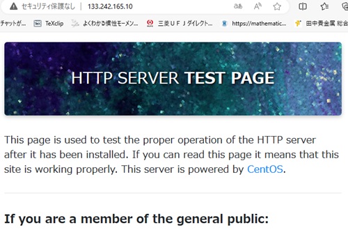
CentOS Stream9 2024インストール – 1
-
IPアドレス
カテゴリー
-
TikZ
カテゴリー
-

コードの組み方
カテゴリー
-
ワイルドカードマスク
カテゴリー

Title Text
Lorem ipsum dolor sit amet, consectetur adipiscing elit, sed do eiusmod tempor incididunt ut labore et dolore magna aliqua.
Title Text
Lorem ipsum dolor sit amet, consectetur adipiscing elit, sed do eiusmod tempor incididunt ut labore et dolore magna aliqua.
Title Text
Lorem ipsum dolor sit amet, consectetur adipiscing elit, sed do eiusmod tempor incididunt ut labore et dolore magna aliqua.
Title Text
Lorem ipsum dolor sit amet, consectetur adipiscing elit, sed do eiusmod tempor incididunt ut labore et dolore magna aliqua.
-
-
diff-eq.comスケールアップマイグレーション3
カテゴリー : diff-eq.comスケールアップマイグレーション3微分方程式いろいろ(https://diff-eq.com)のスケールアップした際の手順のログの第3回目になり…
-
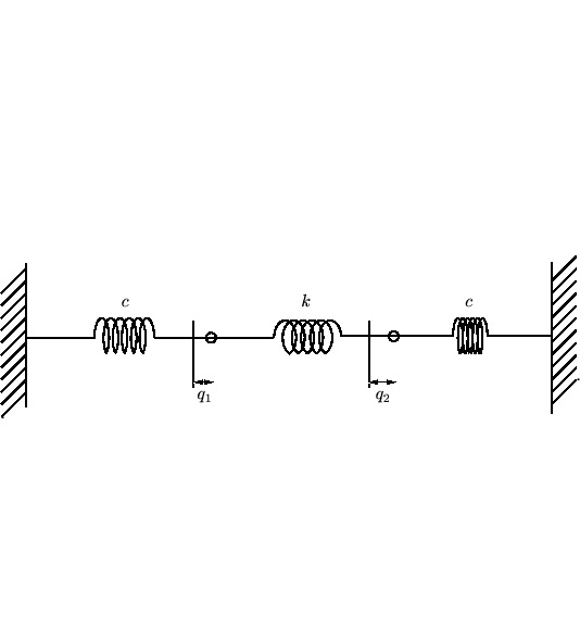
連成振動の解②━LaTeXコード置き場
カテゴリー : 連成振動の解②LaTeXコード微分方程式いろいろコンテンツ“連成振動の解②(3重ばねの振動)”にて使われたLaTeXコード置き場になります。…
-
diff-eq.comスケールアップマイグレーション2
カテゴリー : diff-eq.comスケールアップマイグレーション2微分方程式いろいろのOSの脆弱性、およびスケールアップに伴うマイグレーションの備忘録、ログになります。
-
diff-eq.comスケールアップマイグレーション1
カテゴリー : diff-eq.comスケールアップマイグレーション1微分方程式いろいろのOSの脆弱性、およびスケールアップに伴うマイグレーションの備忘録、ログになります。
-
-
WordPressカテゴリ作成と配置方法
カテゴリー : WordPressカテゴリ作成と配置方法このエントリーではWordPressにてデフォルトで作成されるcategoryのプラグインによる削除と新規で作…
-
CentOS Stream9 2024インストール – 1
カテゴリー : CentOS Stream9 2024インストール – 12024年CentOSの最新版Stream9のさくらサーバでの実装手順になります。途中Puttyが動かなくなる…
-
-